library(tidyverse)
library(shiny)Introduction
This week’s TidyTuesday explores the connections between sister cities across the globe. Unlike previous posts, this one is going to use shiny to create an interactive app.
In particular, I’m interested in identifying chains of sister cities that connect two countries.
Setup
Loading the Data
# tuesdata <- tidytuesdayR::tt_load('2026-05-12')
# cities   <- tuesdata$cities |>
#   write_csv("cities.csv")
# links    <- tuesdata$links |>
#   write_csv("links.csv")

cities <- read_csv("cities.csv")
links  <- read_csv("links.csv")
Distance chain finding algorithm
To find the connection between two cities, we can treat the sister city relationships as an undirected graph. The following function uses the igraph package to find the the number of links in the shortest path between any two city codes. I’m also creating a tall version of this for different kinds of visualizations.
library(igraph, warn.conflicts = FALSE)

links_graph <- graph_from_data_frame(links, directed = FALSE)
distances <- distances(links_graph)

distances <- as_tibble(distances)

distances_tall <- distances |>
  pivot_longer(everything(), names_to = "to", values_to = "distance") |>
  mutate(from = rep(names(distances), ncol(distances)))
number_of_connections <- distances_tall |>
group_by(from) |>
summarise(total_connections = sum(distance > 0 & distance != Inf))
ggplot(number_of_connections |>
mutate(total_connections = as.factor(total_connections)), aes(x = total_connections)) +
geom_histogram(stat = "count") Warning in geom_histogram(stat = "count"): Ignoring unknown parameters:
`binwidth` and `bins`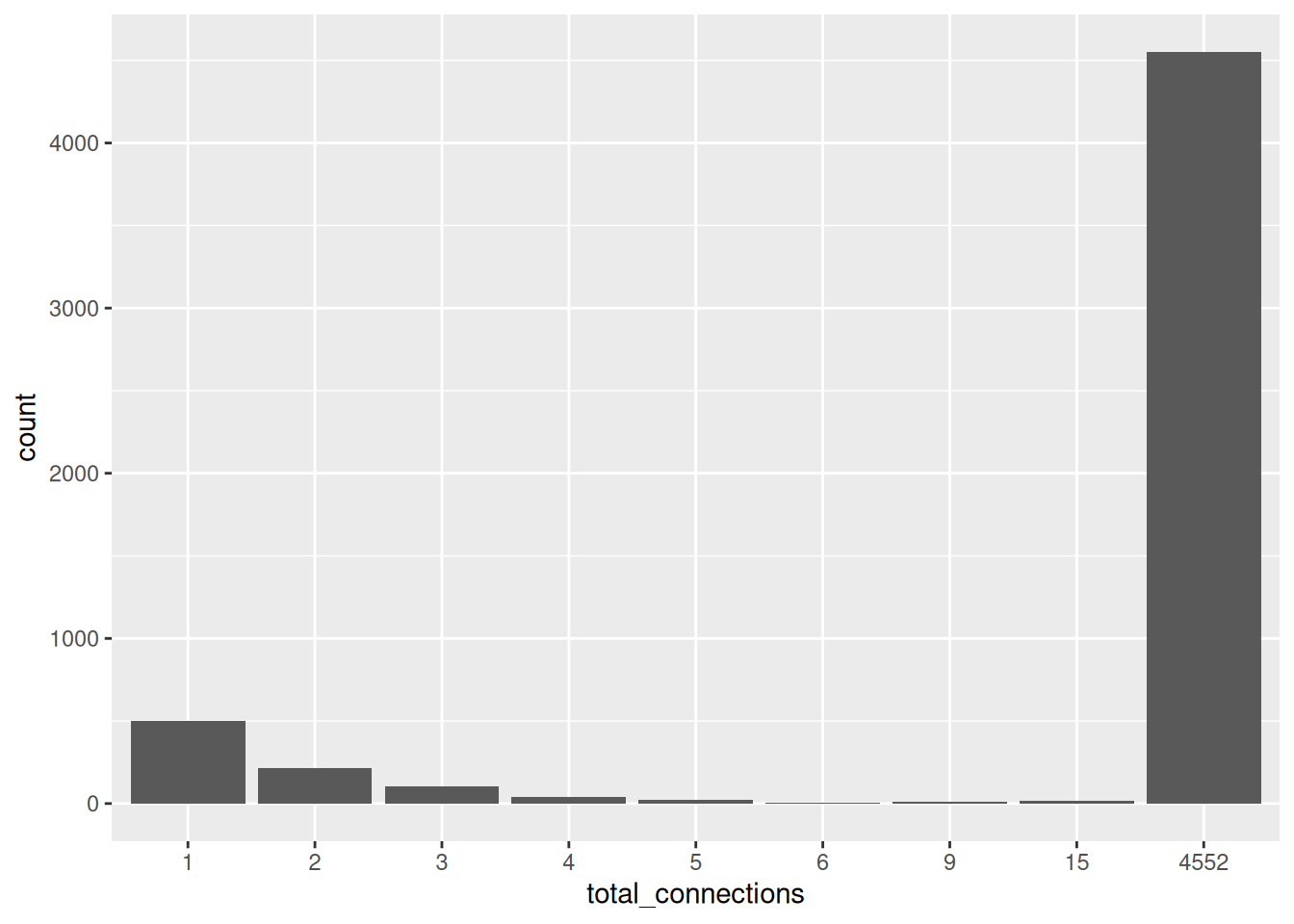
It looks like there is one giant web of 4552 sister cities and a cluster of isolated smaller webs.
ggplot(distances_tall, aes(x = distance)) +
  geom_histogram()
`stat_bin()` using `bins = 30`. Pick better value `binwidth`.Warning: Removed 9188278 rows containing non-finite outside the scale range
(`stat_bin()`).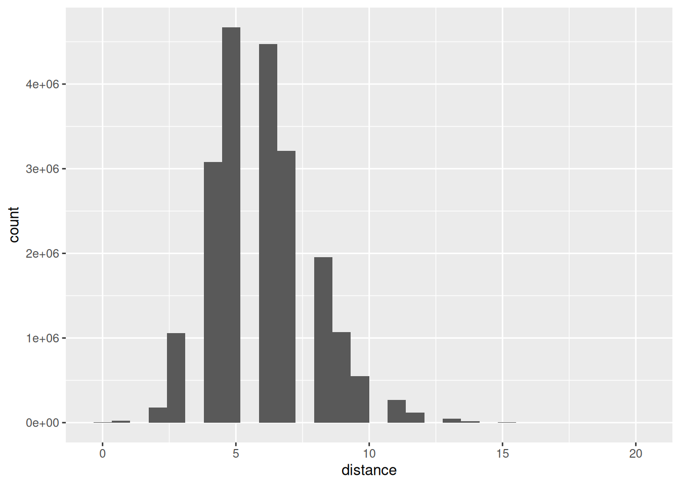
Let’s connect the city ids to the remaining data and see if we can identify some additional patterns
number_of_connections_detail <- number_of_connections |>
  left_join(cities, by = c("from" = "id")) |>
  mutate(is_isolated = total_connections != 4552)

connections_formula_location <- is_isolated ~  lng + lat
number_of_connections_detail |>
  glm(connections_formula_location, family = "binomial", data = _ ) |>
  summary()
Call:
glm(formula = connections_formula_location, family = "binomial",
    data = number_of_connections_detail)

Coefficients:
              Estimate Std. Error z value Pr(>|z|)
(Intercept) -2.9923457  0.1433680 -20.872   <2e-16 ***
lng         -0.0009952  0.0006021  -1.653   0.0984 .
lat          0.0335798  0.0031144  10.782   <2e-16 ***
---
Signif. codes:  0 '***' 0.001 '**' 0.01 '*' 0.05 '.' 0.1 ' ' 1

(Dispersion parameter for binomial family taken to be 1)

    Null deviance: 4946.3  on 5469  degrees of freedom
Residual deviance: 4773.5  on 5467  degrees of freedom
AIC: 4779.5

Number of Fisher Scoring iterations: 5
It looks like the further South you go, the more likely you are to be part of the giant network of cities. Taking this a step further, let’s plot all the latitudes and longitudes and categorize them by the number of connections.
ggplot(data = number_of_connections_detail |> mutate(total_connections = as.factor(total_connections)), aes(x = lng, y = lat, color = total_connections)) +
  geom_point() +
  theme(legend.position = "bottom") +
  scale_color_brewer(palette = "Set1")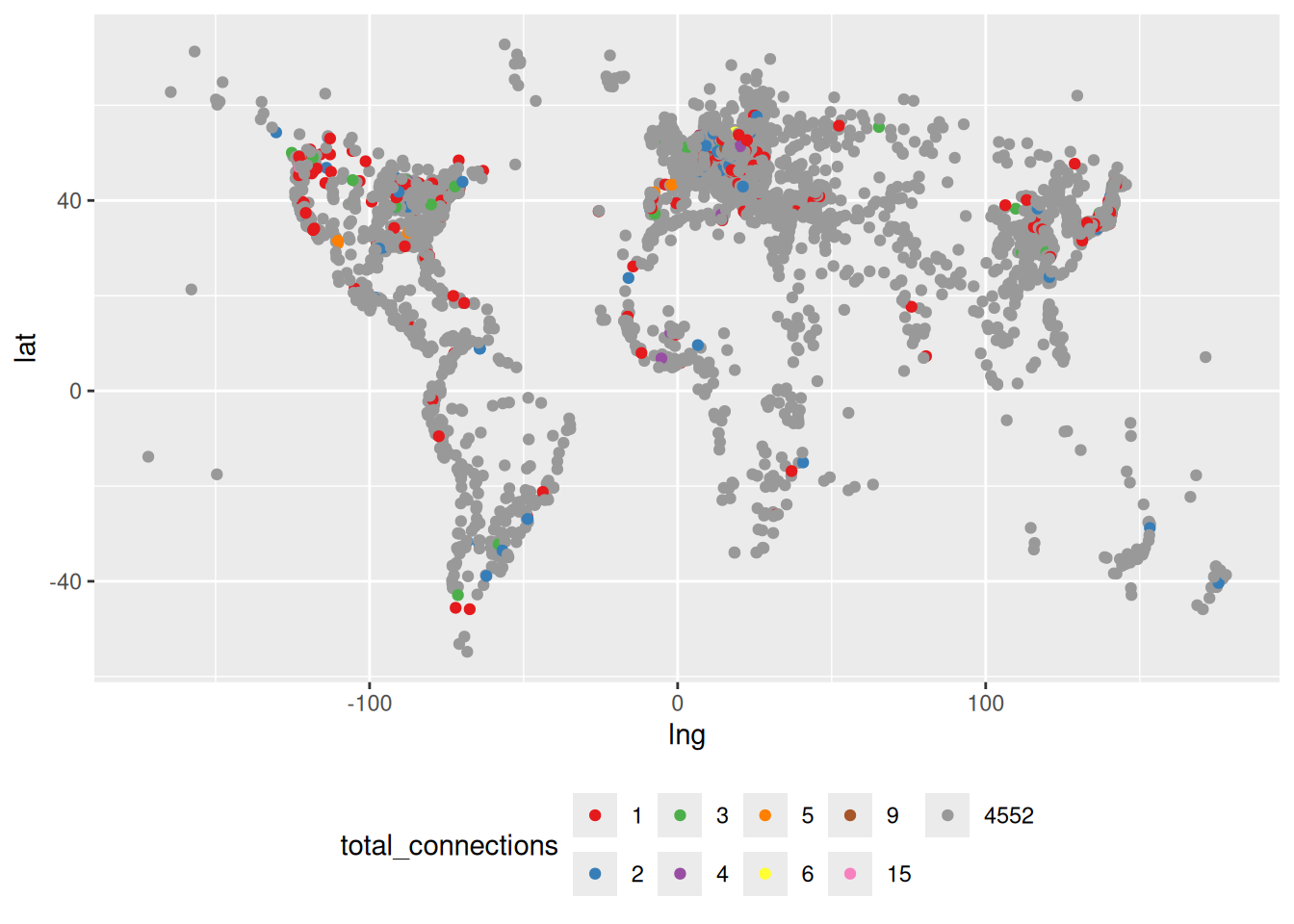
Instead of just highlighting the isolated cities, let’s actually connect them.
links_detail <- links |>
  left_join(cities |> select(id, lng, lat), by = c("source" = "id")) |>
  rename(from_lng = lng, from_lat = lat) |>
  left_join(cities |> select(id, lng, lat), by = c("target" = "id")) |>
  rename(to_lng = lng, to_lat = lat) |>
  left_join(number_of_connections_detail |> select(from, is_isolated, total_connections),  by= c("source" = "from"))

ggplot(data = links_detail) +
  geom_point(aes(x = from_lng, y = from_lat), color = "grey", alpha = 0.2) +
  geom_segment(data = links_detail |> filter(total_connections <=3), mapping = aes(x = from_lng, y = from_lat, xend = to_lng, yend = to_lat, color = as.factor(total_connections))) +
  theme(legend.position = "bottom")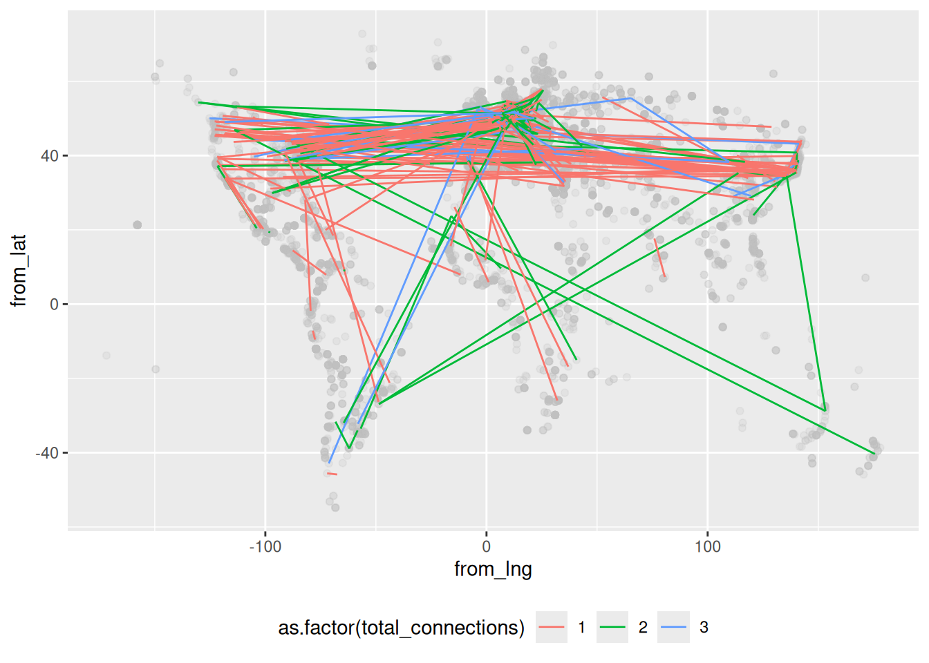
It looks like a mess at the top, but clearly being in the south means you are way less likely to have a small network of sister cities.