Tidy Tuesday: Predicting Castles, Fortresses, and Palaces

Introduction

This week’s Tidy Tuesday dataset features world castles, fortresses, palaces, and ruins. These historical structures span centuries and continents. In this post, we’ll build a predictive model to classify the type of site using its latitude and longitude and the year it was constructed or first documented. Both geography and year help us pinpoint the specific civilization as well as whether we are at nearer the rise or collapse of that civilization and therefore, whether it is likely to be a ruin.

We will use the tidymodels framework in R to build a random forest classifier.

Loading the Data

Let’s start by loading the necessary libraries and the dataset. I’m making one modification to our data by filtering out the ruins. The spirit of our prediction is that our input variables give us information about circumstances around their creation. No one creates a ruin; it’s the destruction of one of the other site types. Therefore, the year in partcular, cannot be a useful predictor.

library(tidyverse)
library(tidymodels)

theme_set(theme_light())

# Load the data
# tuesdata <- tidytuesdayR::tt_load('2026-09-01')
# sites <- tuesdata$world_castles
# write.csv(sites, "sites.csv", row.names = FALSE)

sites <- read.csv("sites.csv") |>
  select(qid, name, category, year, lat, lon) |>
filter(category != "ruin")

head(sites)

       qid                  name category year      lat       lon
1   Q12501   Great Wall of China fortress -700 40.43139 116.56444
2    Q2946  Palace of Versailles   palace 1661 48.80472   2.12028
3   Q80290        Forbidden City   palace 1420 39.91583 116.39083
4 Q1143049 Château de Montsoreau   castle  990 47.21560   0.06220
5  Q131013   Acropolis of Athens fortress -500 37.97167  23.72611
6  Q133274               Kremlin fortress 1420 55.75167  37.61778

Exploratory Data Analysis

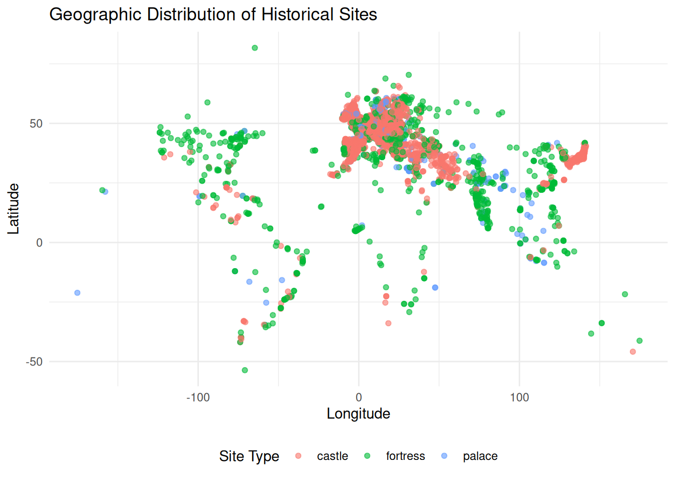
Before building the model, let’s visualize the distribution of our historical sites.

ggplot(sites, aes(x = lon, y = lat, color = category)) +
  geom_point(alpha = 0.6) +
  labs(title = "Geographic Distribution of Historical Sites",
       x = "Longitude",
       y = "Latitude",
       color = "Site Type") +
  theme_minimal() +
  theme(legend.position = "bottom")

It looks like there is some geographical concentration of various site types.

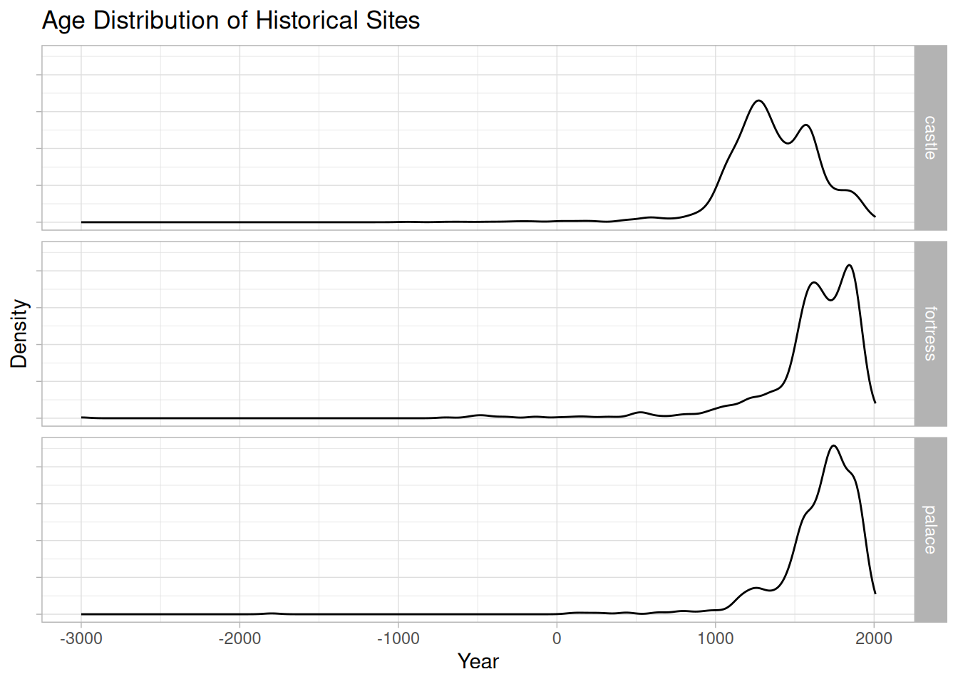
Now let’s look at the distribution of the construction year by site type.

ggplot(sites, aes(x = year)) +
  geom_density(alpha = 1) +
  labs(title = "Age Distribution of Historical Sites",
       x = "Year",
       y = "Density") +
  facet_grid(rows = vars(category)) + 
  theme(axis.text.y = element_blank())

It looks like castles and ruins tend to older than fortresses and palaces.

Building the Model with tidymodels

We’ll predict category using year, lat, and lon.

Data Splitting and Resampling

set.seed(42)
site_split <- initial_split(sites, strata = category)
site_train <- training(site_split)
site_test <- testing(site_split)
site_folds <- vfold_cv(site_train, strata = category)

Creating the Recipe and Model Specification

A random forest model is commonly used for classification with more than two classes. In this case we have four.

site_rec <- recipe(category ~ year + lat + lon, data = site_train)

rf_spec <- rand_forest(trees = 500, min_n = tune(), mtry = tune()) |>
  set_engine("ranger", importance = "impurity") |>
  set_mode("classification")

site_wf <- workflow() |>
  add_recipe(site_rec) |>
  add_model(rf_spec)

Tuning the Model

Let’s tune the hyperparameters of our random forest.

rf_res <- tune_grid(
  site_wf,
  resamples = site_folds,
  grid = 10,
  control = control_grid(save_pred = TRUE)
)

# Select the best model based on accuracy
best_rf <- select_best(rf_res, metric = "accuracy")

# Finalize the workflow
final_wf <- finalize_workflow(site_wf, best_rf)

Final Evaluation

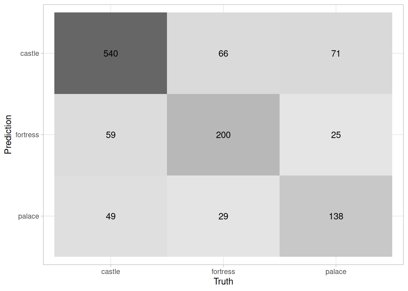
Now, let’s fit our final model to the training data and evaluate it on the testing set.

final_fit <- last_fit(final_wf, site_split)

collect_metrics(final_fit)

# A tibble: 3 × 4
  .metric     .estimator .estimate .config        
  <chr>       <chr>          <dbl> <chr>          
1 accuracy    multiclass     0.746 pre0_mod0_post0
2 roc_auc     hand_till      0.870 pre0_mod0_post0
3 brier_class multiclass     0.177 pre0_mod0_post0

Let’s visualize the confusion matrix to see where our model succeeds and where it gets confused.

collect_predictions(final_fit) |>
  conf_mat(category, .pred_class) |>
  autoplot(type = "heatmap")

Conclusion

In this post, we demonstrated how to use the tidymodels framework to classify historical sites based on their location and age.